From Recurrent Networks to Transformers, How Attention Changed Everything

This is part 1 of 2

What is natural language and how do we make machines speak our language?

Natural language is how humans communicate be it through words, sentences, or context. Teaching machines to understand and generate human language is one of the most challenging problems in AI, since machines only understand numbers or 0 and 1’s.

The Problem with Traditional Approaches

Before Transformers (the model that powers GPT) we used:

1. RNNs (Recurrent Neural Networks): Process text word by word, but struggle with long sequences
2. LSTMs (Long-Short Term Memory): Better at handling long-term dependencies, but still sequential
3. GRUs (Gated Recurrent Unit): Faster than LSTMs but similar limitations

Let’s go over them one by one

Recurrent Neural Networks

Traditional Neural Networks

When you think about traditional neural networks, which I covered in depth here

Basically, we go from input X which we then multiply with the weight matrix and apply the activation function and keep continuing this process to get the output Y.

$$Y = \sigma(f_{(L-1)}(\dots f_1(x)))$$

source : https://goodboychan.github.io/images/simpleRNN.png

How RNNs carry over context

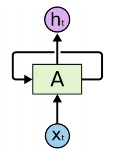
The novel thing about the RNNs and how they in their time revolutionized natural language. They introduced a feedback loop into each cell - which would basically add the information from all the previous layers.

Consider the following architecture of a simple RNN architecture for a stock price predictor with 3 days worth of data:

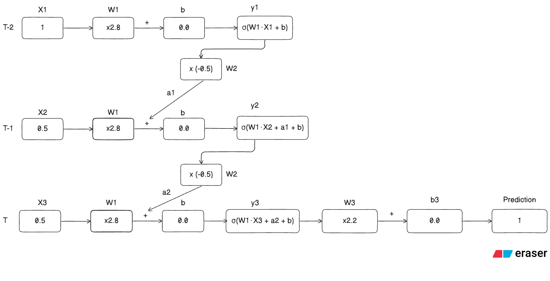
Note: The weights and biases for all the three timesteps are the same, this is the novelty of this network which helps carry over context to the next timestep

What’s happening in the given architecture

$$\sigma = \text{activation function}$$

Step 1: for timestamp T-2 we calculate the activation for input $X_1$,

$$y_1 = \sigma(W_1 \cdot X_1 + b)$$

for the feedback loop we calculate the following,

$$a_1 = y_1 \times W_2$$

Step 2: for timestamp T-1 we calculate the activation for input $X_2$ and add the activation $a_1$,

$$y_2 = \sigma(W_1 \cdot X_2 + a_1 + b)$$

for the feedback loop we calculate the following,

$$a_2 = y_2 \times W_2$$

Step 3: for timestamp T we calculate the activation for input $X_3$ and add the activation $a_2$,

$$y_3 = \sigma(W_1 \cdot X_3 + a_2 + b)$$

Step 4: Calculate the prediction with a simple feed forward operation,

$$output = \sigma(W_3 \cdot y_3 + b_3)$$

Note: The activation for the final layer depends on the kind of task you are trying to perform,

• Linear: Regression
• Sigmoid: Binary classification
• Softmax: Multi-class classification

Note: We usually use tanh function for the hidden state in a RNN network

Why we usually don’t use RNN’s anymore

Exploding OR Vanishing Gradients

1. Exploding Gradients

Imagine W2 to be a constant number for now,

$$W_2 = 4$$

Now imagine we have 100 timesteps (which still isn’t a lot of data to train a decent RNN) the final layer becomes,

$$y_{100} = 4^{100} \cdot X_{100} + b \\ 4^{100} = 1.606938 \cdot {10^{60}}$$

Now, these huge values creep into the gradients we calculate during gradient descent and will eventually “explode” them and will make it harder for the gradient descent algorithm to converge since we take bigger steps in the update rule.

$$W_{new} = W_{old} - \alpha \frac{\partial J}{\partial W}$$

2. Vanishing Gradients

Similarly, Imagine W2 to be a constant number for now,

$$W_2 = 0.2$$

Now imagine we have 100 timesteps (which still isn’t a lot of data to train a decent RNN) the final layer becomes,

$$y_{100} = (0.2)^{100} \cdot X_{100} + b \\ (0.2)^{100} = 1.2676506 \cdot 10^{-70} \approx 0$$

Similarly, these extremely small creep into the gradients we calculate during gradient descent and will eventually make them “vanish” and make it harder for the gradient descent algorithm to converge since we take almost don’t change our W values

$$W_{new} = W_{old} - \alpha \frac{\partial J}{\partial W}$$

To solve these we came up with the LSTM network or the Long-Short Term Memory Network.

Long-Short Term Memory Networks

Now, let’s look at a model that tried to solve the vanishing / exploding gradient problem.

The main idea behind the LSTM is to add 2 different pathways for long-term and short-term memories.

How it tackles exploding / vanishing gradients problem? The long-term memory pathway lacks weights and biases which avoids the said problem.

Before we dive into the LSTM architecture let’s see what the hadamard product is

$$\begin{bmatrix} a_1 \\ a_2 \\ a_3 \end{bmatrix} \odot \begin{bmatrix} b_1 \\ b_2 \\ b_3 \end{bmatrix} = \begin{bmatrix} a_1 \times b_1 \\ a_2 \times b_2 \\ a_3 \times b_3 \end{bmatrix}$$

It’s basically element wise multiplication.

The Architecture

Stage 1 : Forget Gate

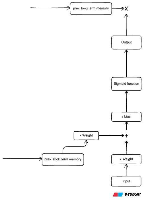
Part 1 - The Math

$$f_t = \sigma(W^x_f \times x_t + W^h_f \times h_{t-1} + b_f)$$ $$\begin{matrix} \sigma = \text{sigmoid function} \in (0, 1) \\ x_t = \text{input at timestep t} \\ W^x_f = \text{Slice of } W_f \text{ for input x} \\ W^h_f = \text{Slice of } W_f \text{ for prev. state} \\ h_{t-1} = \text{prev. short term memory} \\ b_f = \text{bias term for this cell} \end{matrix}$$ $$C_f = f_t \odot C_{t-1}$$ $$\begin{matrix} C_t = \text{curr. timestep long-term memory} \\ C_{t-1} = \text{prev. timestep long-term memory} \\ f_t = \text{forget gate output for curr. timestep} \end{matrix}$$

Note: We assume this to be the first LSTM cell, and hence there is no contribution from the previous cell. This will be clearer once you understand all the gates in a LSTM network.

Part 2.1 - What’s happening?

The first stage determines what percentage of the long-term memory should be “forgotten”, hence the name. This is because the output of the sigmoid function lies between 0 and 1. When this value is multiplied by the previous timestep’s long-term memory, it decides how much information is retained and how much is discarded.

Part 2.2 - Cases

Case 1: Input which results in activation close to 0

This would result in the result to become 0, that implies we completely forget the long-term memory to this point in the network

Case 2: Input which results in activation closer to 1

The more the activation is closer to 1, the less the long-term memory is updated.

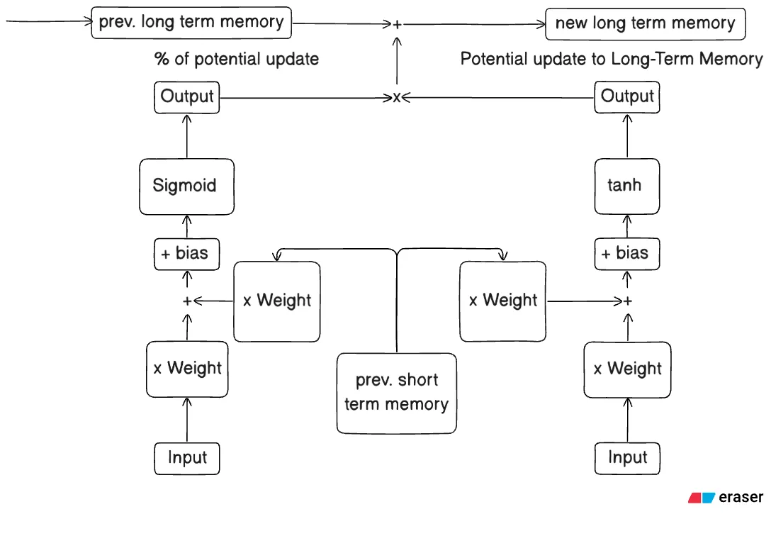
Stage 2 : Input Gate

Part 1.1 - The Math - candidate cell (right)

$$\tilde C_t = \tanh(W^x_c \times x_t + W^h_c \times h_{t-1} + b_c)$$ $$\begin{matrix} \tanh = \text{tanh function} \in (-1, 1) \\ W^x_c = \text{Slice of } W_c \text{ for input x} \\ W^h_c = \text{Slice of } W_c \text{ for prev. state} \\ h_{t-1} = \text{prev. short term memory} \\ b_c = \text{bias term for this candidate cell} \end{matrix}$$

Part 1.2 - The Math - sigmoid cell (left)

$$i_t = \sigma(W^x_i \times x_t + W^h_i \times h_{t-1} + b_i)$$ $$\begin{matrix} \sigma = \text{sigmoid function} \in (0, 1) \\ x_t = \text{input at timestep t} \\ W^x_i = \text{Slice of } W_i \text{ for input x} \\ W^h_i = \text{Slice of } W_i \text{ for prev. state} \\ h_{t-1} = \text{prev. short term memory} \\ b_i = \text{bias term for this sigmoid cell} \end{matrix}$$

Part 1.3 - The Math - Final computation

$$C_t = \tilde C_t \odot i_t + C_f$$ $$\begin{matrix} C_t = \text{updated long-term memory} \\ i_t = \text{sigmoid cell output for input gate} \\ \tilde C_t = \text{candidate cell output for input gate} \\ C_f = \text{prev. long-term memory OR output from forget gate} \\ \end{matrix}$$

Part 2 - What’s happening?

Each input gate has 2 cells - candidate or tanh cell and sigmoid cell. The candidate cell calculates the potential update to the Long-Term Memory and the sigmoid cell calculates the percentage of the potential update that actually goes through.

Part 2.1.1 - Candidate Cell (Right)

This cell is responsible for calculating the potential effect this set of input, short-term memory, weight and bias will have on the Long-Term Memory.

Part 2.1.2 - Sigmoid Cell (Left)

This cell is responsible for calculating the percentage of the potential memory to save or update the Long-Term Memory given a set of input, short-term memory, weight and bias.

Part 2.2 - Cases

Case 1.1: tanh activation produces a negative value

This would negatively influence the Long-Term Memory given the sigmoid cell ≠ 0

Case 1.2: tanh activation produces a positive value

This would positively influence the Long-Term Memory given the sigmoid cell ≠ 0

Case 1.3: sigmoid activation produces a value of 0

This would not influence the Long-Term Memory at all since the sigmoid cell = 0

Stage 3 : Output Gate

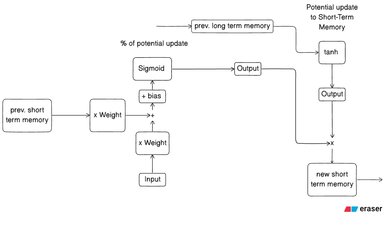
Part 1.1 - The Math - sigmoid cell (left)

$$O_t = \sigma(W^x_o \times x_t + W^h_o \times h_{t-1} + b_o)$$ $$\begin{matrix} \sigma = \text{sigmoid function} \in (0, 1) \\ x_t = \text{input at timestep t} \\ W^x_o = \text{Slice of } W_o \text{ for input x} \\ W^h_o = \text{Slice of } W_o \text{ for prev. state} \\ h_{t-1} = \text{prev. short term memory} \\ b_o = \text{bias term for this sigmoid cell} \end{matrix}$$

Part 1.2 - The Math - candidate cell (right)

$$C_o = \tanh(C_t)$$ $$\begin{matrix} \tanh = \text{tanh function} \in (-1, 1) \\ C_o = \text{candidate output - output gate} \\ C_t = \text{updated long-term memory from input gate} \end{matrix}$$

Part 1.3 - The Math - Final computation

$$h_t = C_o \odot O_t$$ $$\begin{matrix} O_t = \text{sigmoid output - output gate} \\ C_o = \text{candidate output - output gate} \\ h_t = \text{updated short-term memory from output gate} \end{matrix}$$

Part 2 - What’s happening?

Each input gate has 2 cells - candidate or tanh cell and sigmoid cell. The candidate cell calculates the potential update to the Short-Term Memory and the sigmoid cell calculates the percentage of the potential update that actually goes through.

Part 2.1.1 - Candidate Cell (Right)

This cell is responsible for calculating the potential effect the long-term memory will have on the Short-Term Memory and hence the output.

Part 2.1.2 - Sigmoid Cell (Left)

This cell is responsible for calculating the percentage of the potential memory to save or update the Short-Term Memory given set of input, prev. short-term memory, weights and bias.

Part 2.2 - Cases

Case 1.1: tanh activation produces a negative value

This would make the Short-Term Memory negative given the sigmoid cell ≠ 0

Case 1.2: tanh activation produces a positive value

This would make the Short-Term Memory positive given the sigmoid cell ≠ 0

Case 1.3: sigmoid activation produces a value of 0

This would return the output of the LSTM unit = 0, since we multiply both activations.

Gated Recurrent Unit Network

GRU in essence is a modified and optimized version of an LSTM network, it uses fewer gates to achieve similar results. The GRU has 2 gates - reset gate and update gate, both the gates have analogous architecture like the input-output gates in an LSTM, just the trainable parameters (weights and biases) vary.

The Architecture

Reset and Update Gate - Analogous Architecture

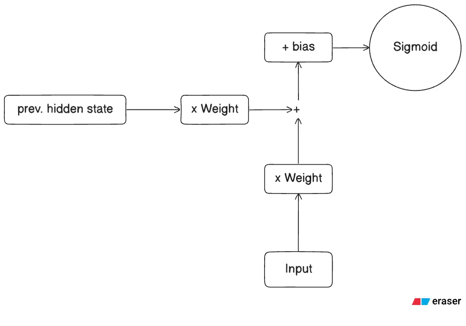
Reset Gate

Part 1 - The Math

$$r_t = \sigma(W^x_r x_t + W^h_r h_{t-1} + b_r)$$ $$\begin{matrix} x_t = \text{input value} \\ b_r = \text{bias for reset gate} \\ W^x_r = \text{Slice of } W_r \text{ for input x} \\ W^h_r = \text{Slice of } W_r \text{ for prev. state} \\ r_t = \text{reset gate value for curr. timestep} \\ \end{matrix}$$

Part 2.1 - What’s happening?

The reset gate controls how much of the previous hidden state to forget.

Part 2.2 - Cases

Case 1.1 If the value is close to 0

It tells the model to completely ignore or “reset” the corresponding information in the previous hidden state. This allows the model to focus on the current input without being distracted by irrelevant past information.

Case 1.2 If the value is close to 1

It allows the model to fully remember that part of the previous hidden state.

Update Gate

Part 1 - The Math

$$z_t = \sigma(W^x_z x_t + W^h_z h_{t-1} + b_z)$$ $$\begin{matrix} x_t = \text{input value} \\ b_z = \text{bias for update gate} \\ W^x_z = \text{Slice of } W_z \text{ for input x} \\ W^h_z = \text{Slice of } W_z \text{ for prev. state} \\ z_t = \text{update gate value for curr. timestep} \\ \end{matrix}$$

Part 2.1 - What’s happening?

The update gate controls how much of the previous hidden state to carry forward.

Case 1.1 If the value is close to 0

It tells the model to primarily update the hidden state with the new candidate information, i.e update everything in a sense.

Case 1.2 If the value is close to 1

It tells the model to carry everything forward and ignore the new candidate state.

How these gates work together?

We first compute an intermediary hidden state called the candidate hidden state or new candidate state using,

$$\tilde h_t=\tanh (W^x_h \times x_t + W^r_h(r_{t} \odot h_{t-1})+b_{h})$$ $$\begin{matrix} x_t = \text{input value} \\ \tilde h_t = \text{candidate hidden state} \\ W^x_h = \text{Slice of } W_h \text{ for input x} \\ b_h = \text{bias for intermediate step} \\ W^r_h = \text{Slice of } W_h \text{ for reset computation} \\ \end{matrix}$$

Now, we will calculate the final hidden state using the update gate,

$$h_t = (1 - z_t) \odot h_{t-1} + z_t \odot \tilde h_t$$

Basically, the final state is an aggregation of how much information of the previous hidden state to preserve + how much information of the new hidden state to carry over

In the next post we will go through the coveted transformer network that powers GPT, Gemini and more.