Introduction: Why do we need neural networks?

Why do we need neural networks? When we start learning about machine learning we learn something called as Logistic Regression, which is a linear model that is used to predict the probability of a binary outcome. So why is that we need neural networks? Simple Answer, since it’s a linear model it cannot model complex relationships.

The Foundation: Linear Algebra, Linear Regression and Logistic Regression

Linear Algebra

Let’s focus our attention on linear algebra for a moment, I promise it will be worth it.

We will focus on matrix multiplication for now.

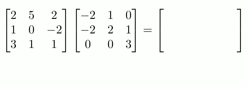
source: https://www.mscroggs.co.uk/img/full/multiply_matrices.gif

Rule: number of columns of 1st matrix = number of rows of the 2nd matrix

Once you’ve made yourself familiar with matrix multiplication, which is core to machine learning, let’s move on. What does matrix multiplication in machine learning actually signify and why do we need it in the first place?

Matrix multiplication represents linear transformations - operations that preserve lines and the origin while scaling and rotating vectors.

In machine learning, we use matrix multiplication to primarily make batch processing (processing multiple units of input simultaneously considering datasets can be in the order of billions) possible.

The other reason is so we can add non-linearity to the linear transformation using an activation function (which we will revisit in the future).

I will keep the next two topics brief,

Linear Regression

We use this algorithm to predict continuous values. It finds the best-fit line through data points by minimizing the sum of squared errors. The model learns weights (w) and bias (b) such that:

$$y = wx + b$$

Linear regression is the foundation upon which more complex models are built, think of it as trying to fit a line through some data points which can later be used to predict the value of y given w, x and b

source: https://gbhat.com/assets/gifs/linear_regression.gif

Logistic Regression

Logistic regression is used for binary classification problems. It applies a sigmoid function (non-linearity) to the linear output to produce probabilities between 0 and 1:

$$P(y = 1) = \sigma(wx + b)$$

Where $\sigma$ is the sigmoid function: $\sigma(z) = \frac{1}{1 + e^{-z}}$

This creates an S-shaped curve that maps any real number to a probability, making it perfect for classification tasks.

source: https://images.spiceworks.com/wp-content/uploads/2022/04/11040521/46-4-e1715636469361.png

The difference

Simply used for different purposes - linear regression is used to predict continuous values while logistic regression is used to predict a probability.

What we have learnt so far

By now we have learnt how to multiply matrices, why we need to multiply matrices, what is linear regression and logistic regression.

Overfitting and Underfitting

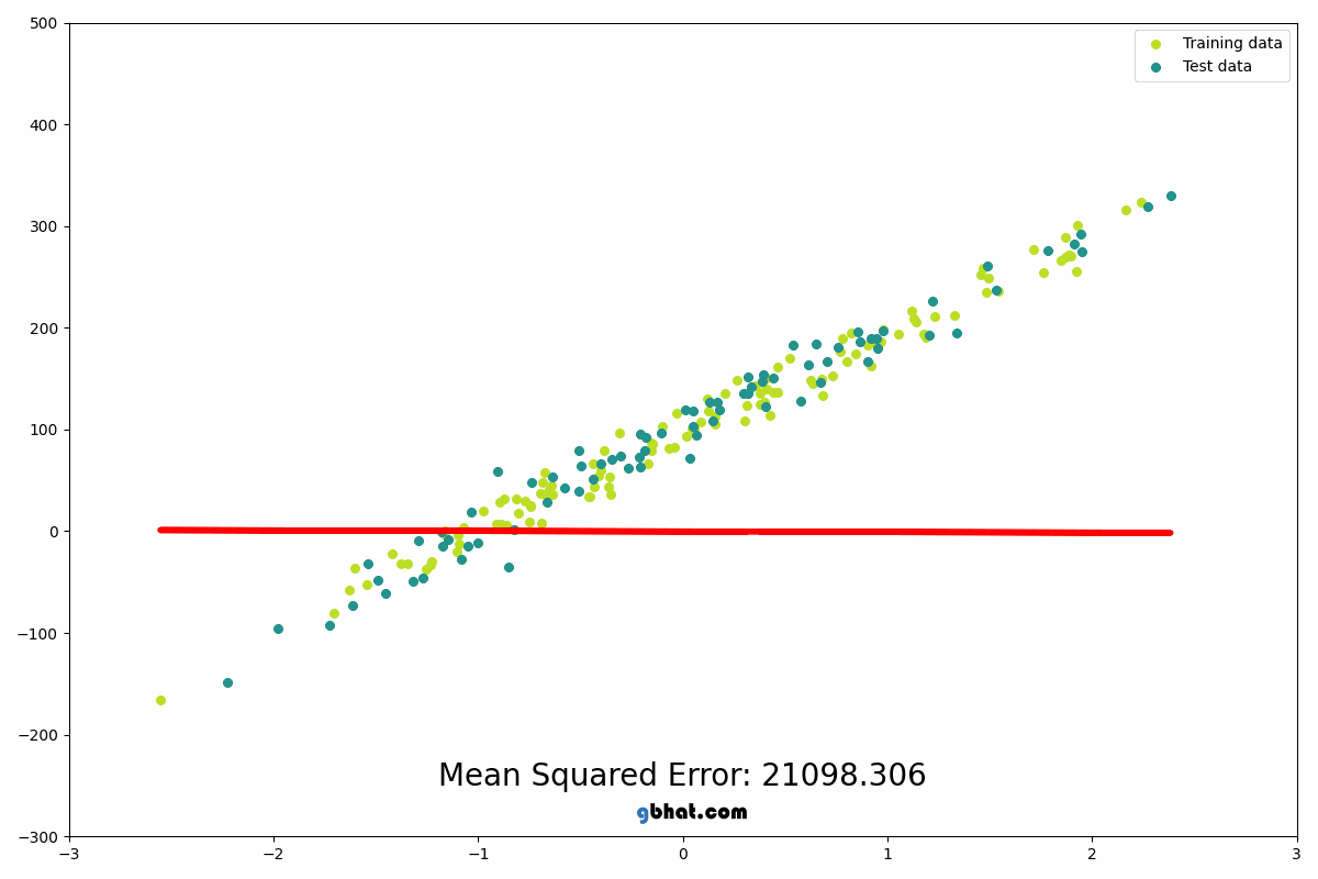
Overfitting

After training, if the model performs well on the training data but doesn’t work well on the testing data, the model has overfit. This means it has memorized the training data instead of learning generalizable patterns.

Underfitting

After training, if the model performs poorly on the training data and also doesn’t work well on the testing data, the model has underfit. This means it hasn’t learned enough from the data and the learnt function is too simple for the problem.

Why This Matters

Understanding overfitting and underfitting is crucial because:

• Overfitting leads to poor generalization on new data
• Underfitting means the model is too simple to capture the underlying patterns
• Finding the right balance is key to building effective neural networks

Neural Networks

A network of nodes

Now let’s dive into the nitty-gritties of Neural Networks. Before we do that we should take a look at how data flows through the network.

source: https://miro.medium.com/v2/resize:fit:1200/1*lGsIwcrmZ960TcvnBWSLwA.gif

I know, I know what even is going on here? Don’t worry we’ll go through each step carefully source: https://y.yarn.co/1ab1e1b9-fd96-426d-b7d6-4d60e8294977_text.gif

Definitions

Now we are going to define some keywords that we are going to use in the future

1. Input Layer: The first layer that receives the raw data (features)
2. Hidden Layer: Intermediate layers between input and output that process the data
3. Output Layer: The final layer that produces the prediction
4. Neuron/Node: Individual processing units in each layer
5. Weight: Parameters that determine the strength of connections between neurons, the higher the weight of some connection the more significance it carries in the network.
6. Bias: Additional parameter that allows the model to shift the activation function
7. Activation Function: Non-linear function applied to the weighted sum of inputs
8. Forward Propagation: Process of passing data through the network from input to output
9. Backward Propagation: Process of updating weights based on prediction errors

How Data Flows Through the Network

Let’s break down what happens in that animated GIF:

1. Input Processing: Raw data enters the input layer
2. Weighted Sum: Each neuron computes $z = wx + b$
3. Activation: Apply activation function: $a = \sigma(z)$
4. Forward Pass: Results flow to the next layer
5. Repeat: Process continues through all hidden layers
6. Output: Final prediction emerges from the output layer

Why did we learn matrix multiplication?

Now we’ll circle back to why we learnt matrix multiplication in the first place,

Consider X to be the input vector $X = \begin{bmatrix}x_1 \\ x_2 \\ x_3\end{bmatrix}$

And W to be the weight matrix $W = \begin{bmatrix}w_{11} & w_{12} & w_{13} \\ w_{21} & w_{22} & w_{23} \\ w_{31} & w_{32} & w_{33}\end{bmatrix}$

When we compute $WX + b$, we’re essentially performing:

$$\begin{bmatrix}w_{11} & w_{12} & w_{13} \\ w_{21} & w_{22} & w_{23} \\ w_{31} & w_{32} & w_{33}\end{bmatrix} \cdot \begin{bmatrix}x_1 \\ x_2 \\ x_3\end{bmatrix} + \begin{bmatrix}b_1 \\ b_2 \\ b_3\end{bmatrix}$$

This helps parallelize the computation by computing a whole batch

The only rule you must follow is that the matrix multiplication should work

1. Matrix-Vector Multiplication: $WX$ gives us the weighted sum for each neuron
2. Bias Addition: Adding $b$ shifts the activation function. This helps prevent overfitting
3. Batch Processing: We can process multiple inputs simultaneously

This is why matrix multiplication is crucial - it allows us to:

• Efficiently compute all neuron outputs in parallel
• Scale to large datasets by processing multiple samples at once
• Vectorize operations for faster computation on GPUs

The beauty is that one matrix multiplication operation can compute the outputs for an entire layer of neurons, making neural networks computationally feasible for real-world applications.

Why Multiple Layers?

The power of neural networks comes from stacking multiple layers:

• Layer 1: Learns simple features (edges, curves)
• Layer 2: Combines simple features into complex patterns
• Layer 3+: Builds increasingly abstract representations

This hierarchical learning allows neural networks to model complex, non-linear relationships that simple linear models cannot capture.

Activation Functions

We briefly mentioned activation functions earlier. Here are the most common ones:

1. Sigmoid: $\sigma(z) = \frac{1}{1 + e^{-z}}$ (0 to 1)
2. ReLU: $f(z) = \max(0, z)$ (fairly popular)
3. Leaky ReLU: $f(z) = \max(0.01z, z)$ prevents dying ReLU problem
4. Tanh: $f(z) = \frac{e^z - e^{-z}}{e^z + e^{-z}}$ (-1 to 1)

Activation functions introduce non-linearity, which is essential for neural networks to learn complex patterns (mapping functions from input to output).

Why Different Activation Functions?

Each activation function has its advantages:

• Sigmoid: Good for probability outputs (0-1 range)
• ReLU: Most popular, computationally efficient, helps with vanishing gradients
• Leaky ReLU: Prevents the “dying ReLU” problem where neurons become inactive
• Tanh: Similar to sigmoid but centered around 0, often better for hidden layers

Training Neural Networks

The Learning Process

Training a neural network involves:

1. Forward Pass: Make predictions using current weights using the following: $y = Wx + b$, and for each layer we add activation to add non-linearity to the mapping function.
2. Loss Function: Is primarily a function to measure the error between the predicted value in the forward pass versus the actual value. We use it to calculate the loss.
3. Backward Pass: Calculate gradients $\nabla(Loss)$ and back propagate the loss by multiplying the gradient with activations and update the weights and bias accordingly.
4. Update Weights: Adjust weights to reduce loss using the gradient descent algorithm.
5. Repeat: Continue until the model performs well

This raises an important question: Why can’t we just find the $\nabla(Loss) = 0$? The simple answer is because the loss function for a neural network is a complex non-linear function and may have multiple local minima which do not represent the most optimal solution for the loss function.

Loss Functions

Common loss functions include:

• Mean Squared Error (MSE): For regression problems
• Cross-Entropy: For classification problems

The choice of loss function depends on your specific problem type.

Gradient Descent and Backpropagation

The core optimization algorithm:

1. Calculate gradients of the loss with respect to each weight, $\frac{\partial L}{\partial w}$
2. Update weights using: $w_{new} = w_{old} - \alpha \cdot \frac{\partial L}{\partial w}$
3. Learning rate $\alpha$ controls how big steps we take. Make sure it’s neither too small (the change step is negligible) nor too large (it might overshoot the most optimal point).

source : https://s3-us-west-2.amazonaws.com/courses-images-archive-read-only/wp-content/uploads/sites/924/2015/11/25201251/CNX_Precalc_Figure_03_02_0032.jpg

Why do we use $-\alpha$ for every iteration and why does it work? There are 2 possible cases:

1. Negative slope - Consider a point on the left side of the function. If we find the slope at point $(1,4)$, we find it to be negative w.r.t. the optimal point $(3,1)$, and if we calculate the update value for $W$ using the update rule, it correctly moves positively towards the optimal point.

2. Positive slope - Consider a point on the right side of the function. If we find the slope at point $(5,4)$, we find it to be positive w.r.t. the optimal point $(3,1)$, and if we calculate the update value for $W$ using the update rule, it correctly moves negatively towards the optimal point.

Hence, for either case, the update rule correctly moves towards the optimal point.

Backpropagation is the algorithm that efficiently computes gradients for all weights in the network:

1. Forward pass: Compute all activations and outputs
2. Compute loss: Calculate the difference between prediction and target
3. Backward pass: Use the chain rule to compute gradients
4. Update weights: Apply gradient descent to all parameters

source : https://miro.medium.com/1*dZNUK-2Zt80rWGM0eP0iEg.gif

What exactly is going on here? Let’s look at the math for a single layer

Consider the following neural network (ignoring the bias term for now), source : https://i.ytimg.com/vi/UJwK6jAStmg/hqdefault.jpg

$$\begin{matrix} \times = \text{scalar multiplication} \\ \cdot = \text{matrix multiplication} \end{matrix}$$

Step 1: Consider the following matrices,

$$X = \begin{bmatrix} x_1 & x_2 \\ \vdots & \vdots\end{bmatrix}_{n\times2} \quad W^{(1)} = \begin{bmatrix}w_{11} & w_{12} & w_{13} \\ w_{21} & w_{22} & w_{23}\end{bmatrix}_{2\times3} \quad W^{(2)} = \begin{bmatrix} w_1 \\ w_2 \\w_3 \end{bmatrix}_{3\times1}$$

Here $n$, defines the number of training samples

Step 2: Calculate activation for 2nd (hidden layer)

$$z^{(2)}_{n\times3} = X_{n\times2} \cdot W^{(1)}_{2\times3}$$ $$a^{(2)}_{n\times3} = \sigma(z^{(2)}_{n\times3})$$

Here, $\sigma$ represents the sigmoid activation function we defined earlier

Step 3: Calculate activation for 3rd (output layer)

$$z^{(3)}_{n\times1} = a^{(2)}_{n\times3} \cdot W^{(2)}_{3\times1}$$ $$\hat{y} = \sigma(z^{(3)}_{n\times1})$$

Here $\hat y$, represents our predictions for the n samples.

Step 4: Define the cost function (for the whole dataset)

$$J = \sum \frac{1}{2}(y - \hat y)^2$$

Step 5: Define the update rule for gradient descent,

$$W^{(1)}_{new} = W^{(1)}_{old} - \alpha \cdot \frac{\partial J}{\partial W^{(1)}}, \quad W^{(2)}_{new} = W^{(2)}_{old} - \alpha \cdot \frac{\partial J}{\partial W^{(2)}}$$

Step 6.1: Let’s find $\frac{\partial J}{\partial W^{(2)}}$,

$$\frac{\partial J}{\partial W^{(2)}} = \frac{\partial \sum \frac{1}{2}(y - \hat y)^2}{\partial W^{(2)}} =\sum -(y - \hat y) \cdot \frac{\partial \hat y}{\partial W^{(2)}}$$ $$\hat{y} = \sigma(z^{(3)}), \quad z^{(3)} = a^{(2)} \cdot W^{(2)}, \quad \frac{\partial \hat y}{\partial W^{(2)}} = \frac{\partial \hat y}{\partial z^{(3)}} \cdot \frac{\partial z^{(3)}}{\partial W^{(2)}}$$

Using Step 3 equations we derive these partials,

$$\frac{\partial \hat y}{\partial z^{(3)}} = \sigma'(z^{(3)}), \quad \frac{\partial z^{(3)}}{\partial W^{(2)}} = a^{(2)}$$

Here, $\sigma '$ represents the derivative of the sigmoid activation function we defined earlier as is defined by,

$$\sigma'(x) = \frac{e^{-x}}{(1 + e^{-x})^2} = \sigma(x) \cdot (1 - \sigma(x))$$

The final form is given by,

$$\frac{\partial J}{\partial W^{(2)}} = -(y - \hat y)_{n\times1} \times \sigma'(z^{(3)})_{n\times1} \cdot a^{(2)}_{n\times3}$$

Scalar multiplication of term 1 and 2 to give,

$$\delta^{(3)}_{n\times1} = -(y - \hat y)_{n\times1} \times \sigma'(z^{(3)})_{n\times1} = \begin{bmatrix} -(y_1 - \hat y_1) \times \sigma'(z_1^{(3)}) \\ -(y_2 - \hat y_2) \times \sigma'(z_2^{(3)}) \\ \vdots \end{bmatrix}_{n\times1}$$

The matrix multiplication form is given by,

$$\frac{\partial J}{\partial W^{(2)}} = a^{(2)T}_{3\times n} \cdot \delta^{(3)}_{n\times1}$$

Step 6.2: Let’s find $\frac{\partial J}{\partial W^{(1)}}$,

$$\frac{\partial J}{\partial W^{(1)}} = \frac{\partial \sum \frac{1}{2}(y - \hat y)^2}{\partial W^{(1)}} =\sum -(y - \hat y) \times \frac{\partial \hat y}{\partial z^{(3)}} \cdot \frac{\partial z^{(3)}}{\partial W^{(1)}} = \delta^{(3)} \cdot \frac{\partial z^{(3)}}{\partial W^{(1)}}$$ $$\frac{\partial z^{(3)}}{\partial W^{(1)}} = \frac{\partial z^{(3)}}{\partial a^{(2)}} \cdot \frac{\partial a^{(2)}}{\partial W^{(1)}} = \frac{\partial z^{(3)}}{\partial a^{(2)}} \cdot \frac{\partial a^{(2)}}{\partial z^{(2)}} \cdot \frac{\partial z^{(2)}}{\partial W^{(1)}}$$

This in essence is chain-rule used to “BACK-PROPAGATE“ the loss

Using Step 2 and 3 equations we derive these partials,

$$\frac{\partial z^{(3)}}{\partial a^{(2)}} = W^{(2)}, \quad \frac{\partial a^{(2)}}{\partial z^{(2)}} = \sigma'(z^{(2)}), \quad \frac{\partial z^{(2)}}{\partial W^{(1)}} = X$$

The final form is given by,

$$\frac{\partial J}{\partial W^{(1)}} = \delta^{(3)}_{n\times1} \cdot W^{(2)}_{3\times1} \cdot \sigma'(z^{(2)})_{n\times3} \cdot X_{n\times2}$$ $$\delta^{(2)}_{n\times3} = \delta^{(3)}_{n\times1} \cdot W^{(2)T}_{1\times3} \times \sigma'(z^{(2)})_{n\times3}$$

The final matrix form is given by,

$$\frac{\partial J}{\partial W^{(1)}} =X^T_{2\times n} \cdot \delta^{(2)}_{n\times3}$$

1. This shows how the error δ flows backward through the activation function and gets multiplied by the input from the previous layer, which is exactly what backpropagation does - it distributes the error back through the network to update the weights.

2. Once you reach the input layer, we can use the gradient descent update rule to update the trainable parameters.

3. If you want to dive deeper into the topic, which I really suggest, read this article: https://medium.com/the-feynman-journal/what-makes-backpropagation-so-elegant-657f3afbbd

Why do we use chain-rule in backpropagation?

The chain rule is essential because neural networks are composite functions: $f(x) = f_L(f_{L-1}(...f_1(x)))$. Where $_L$ defines the layer of the neural network. To compute gradients for weights in earlier layers, we need to understand how changes affect the final loss through all subsequent layers.

By the chain rule: $\frac{\partial L}{\partial w_1} = \frac{\partial L}{\partial f_L} \cdot \frac{\partial f_L}{\partial f_{L-1}} \cdot ... \cdot \frac{\partial f_1}{\partial w_1}$

This allows backpropagation to efficiently compute all gradients in one backward pass, making training of deep networks computationally feasible.

Think of it as accumulating all the loss to the first layer, which makes the algorithm much more efficient.

Conclusion

Neural networks are powerful models that can learn complex patterns by stacking multiple layers of neurons. They build upon the concepts we learned earlier:

• Matrix multiplication for efficient computation
• Linear transformations as the foundation
• Non-linear activation functions for complexity
• Proper training to avoid overfitting and underfitting

The key insight is that neural networks are essentially multiple logistic regression models stacked together, with each layer learning increasingly complex representations of the data.

Understanding overfitting and underfitting helps us build models that generalize well to new data, while the mathematical foundation of matrix operations makes these complex models computationally feasible.

In the next post, we’ll dive deeper into the paper that made ChatGPT what it is today.

References

Images and Animations Used

1. Matrix Multiplication Animation - Matrix Multiplication GIF

2. Linear Regression Visualization - Linear Regression GIF

3. Sigmoid Function Graph - Sigmoid Function Image

4. Neural Network Data Flow - Neural Network Flow GIF

5. The Office GIF - Reaction GIF

6. Neural Network for Backpropagation - https://i.ytimg.com/vi/UJwK6jAStmg/hqdefault.jpg

7. Backpropagation Visualization - Backpropagation GIF

Additional Resources

• Mathematical Notation: All mathematical formulas are rendered using KaTeX