Part 2 of 2

Motivation for Convolutional Neural Networks

As we discussed in the previous blog post, linear classifiers lose spatial information as we convert a 2D spatially aware collection of pixels into a deconstructed 1D spatially unaware vector of pixels.

What exactly is convolution in computer vision?

Instead of deconstructing the image into a 1D vector, we instead slide a kernel (or filter) through the image and taking dot products between the kernel and the small region in the image. The dot product “activates” or highlights specific patterns like edges, corners, etc.

What is the convolution operation?

source : https://miro.medium.com/v2/resize:fit:1052/0*ft0xqDy5VBYTuchD.gif

At each location, the kernel’s values are element-wise multiplied with the corresponding pixel values in the image patch, and all products are summed to create a single output value. The kernel then shifts by a specified number of pixels (called stride) and repeats this process across the entire image.

How is this different or better compared to linear classifiers? fully connected layers treat all pixels equally, convolution focuses on small neighborhoods of pixels at a time, preserving spatial relationships. Additionally, the same kernel weights are reused across the entire image leading to parameter sharing

Let’s define some terms we’re going to use

• Stride - number of pixels by which the kernel (or filter) slides by

• Padding - number of pixel layers added around the border of the input image before applying the convolution operation. This prevents the output feature map from shrinking and preserve information at the image edges.

Let’s solve an example

Consider the following matrices for the image(I) and filter(f),

$$I = \begin{bmatrix} 1 & 0 & 1 & 0 & 1 \\ 0 & 1 & 0 & 1 & 0 \\ 1 & 0 & 2 & 0 & 1 \\ 0 & 1 & 0 & 1 & 0 \\ 1 & 0 & 1 & 0 & 1 \end{bmatrix} \quad f = \begin{bmatrix} -1 & -1 & -1 \\ -1 & 8 & -1 \\ -1 & -1 & -1 \\ \end{bmatrix}$$

If we take the dot product and stride the filter we get the following output,

$$O = \begin{bmatrix} 3 & -5 & 3 \\ -5 & 12 & -5 \\ 3 & -5 & 3 \\ \end{bmatrix}$$

Let’s look at one of the computations and the rest, you can try for yourselves?

$$\begin{bmatrix} 1 & 0 & 1 \\ 0 & 1 & 0 \\ 1 & 0 & 2 \\ \end{bmatrix} \circledast \begin{bmatrix} -1 & -1 & -1 \\ -1 & 8 & -1 \\ -1 & -1 & -1 \\ \end{bmatrix} = (-1 + 0 - 1 + 0 + 8 + 0 - 1 + 0 - 2) = 3$$

this computation is the output for the top left element in the convolved output.

How to calculate output dimensions of the convolution operation

$$O_{dim} = \left\lfloor \frac{n + 2p - f}{s}\right\rfloor+1, \quad \lfloor \rfloor \implies \text{floor function}$$

here, n → input image dims, p → padding, f → filter size, s → stride.

Consider the following example, n = (5 x 5), p = 1, f = (3 x 3), s = 1

$$O_{dim} = \left\lfloor \frac{5 + 2(1) - 3}{1}\right\rfloor+1 = (5 \times 5)$$

Pooling

This is when we downsample higher spatial dimensional information into the most important features, this also makes the architecture computationally efficient to train. Similar to convolution, we have a fixed filter that slides over the input image but instead of computing weighted sums, pooling applies a simple aggregation function like taking the maximum or average value from each region

1. Max Pooling - We take the max or the most important feature of the sub-region.

2. Average Pooling - We compute the mean of values in each region, providing a smoothed representation that captures general patterns rather than sharp features.

   source : https://miro.medium.com/v2/resize:fit:1400/1*WvHC5bKyrHa7Wm3ca-pXtg.gif

Pooling - Example

$$I = \begin{bmatrix} 1 & 3 & 2 & 1 \\ 2 & 9 & 1 & 1 \\ 1 & 3 & 2 & 3 \\ 5 & 6 & 1 & 2 \\ \end{bmatrix}, \quad filter = (2\times2), \ stride = 2$$ $${max\_pool} = \begin{bmatrix} 9 & 2 \\ 6 & 3 \\ \end{bmatrix}, \ {avg\_pool} = \begin{bmatrix} 3.75 & 1.25 \\ 3.75 & 3 \\ \end{bmatrix}$$

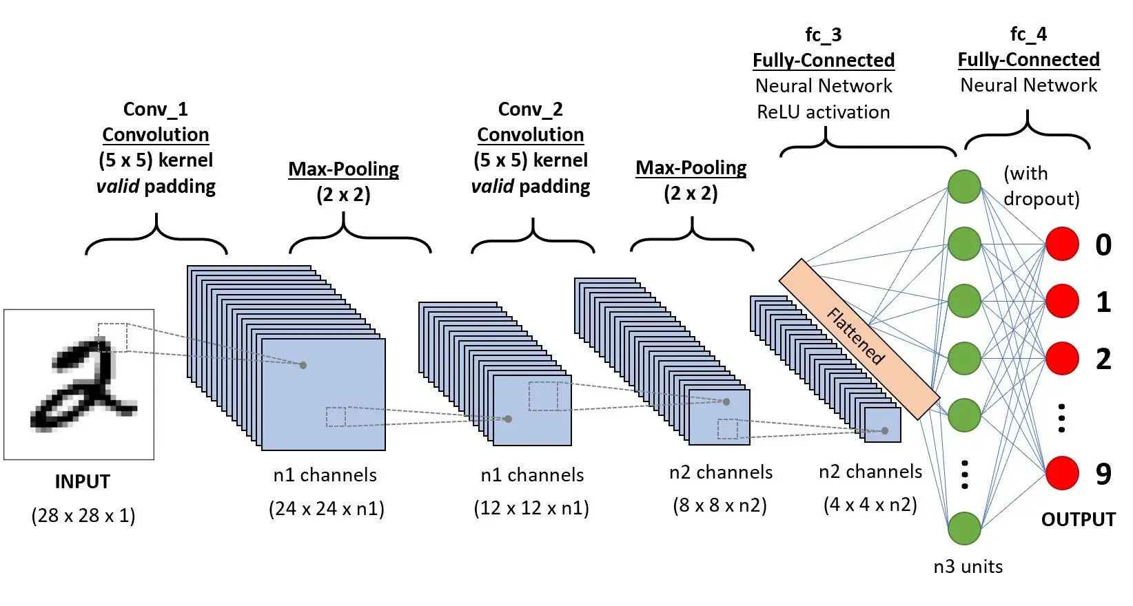
Architecture

source : https://dev-to-uploads.s3.amazonaws.com/uploads/articles/sbrqoqoksznalhywylm3.png

Input Layer

Input layer receives the raw image as a 2D array for grayscale images or 3D tensors for colored images of the form (height x width x channels).

Convolution Blocks

These blocks form the main feature extractor component of the architecture, this is usually repeated multiple times with increasing depth. Each block has multiple components

1. Convolution layers apply learnable filters to detect features like edges, corners, textures and patterns.

2. Activation function (usually ReLU) introduces non-linearity so the model can learn complex non-linear functions

3. Pooling layers (max or average) downsample the learnt feature maps into smaller matrices that retain the most important information while reducing dimensionality and making it easier and more efficient to train.

Flattening Layer

Converts the final 3D feature maps into a 1D vector, preparing the data for classification.

Fully Connected Layers

Combine all the learnt features to understand high level relationships and patterns across the entire image

Output Layer

Final predictions using softmax (for multi-class classification) or sigmoid (for binary classification) activation functions. This layer basically converts the learnt high level relationships and patterns into a probability distribution which can be later used to make a prediction.

Training, Testing

Training and testing is done similar to a linear neural network, we have some training data, testing data, corresponding labels, a loss function (usually cross-entropy), learning rate, an optimizer (usually Adam). In this blog we will explain the code behind training a simple convolutional neural network to learn to predict the MNIST dataset. We will skip explanations for overlapping code from the previous blogpost.

Code

import torch

import torchvision
import torch.nn as nn
import torch.optim as optim
from torch.utils.data import DataLoader
import torchvision.transforms as transforms

import numpy as np
import matplotlib.pyplot as plt

device = torch.device('cuda' if torch.cuda.is_available() else 'cpu')
print(f'Using device: {device}')

1. importing necessary libraries

2. setting the device we will train the network on

transform = transforms.Compose([
transforms.ToTensor(),
transforms.Normalize((0.1307,), (0.3081,))
])

train_dataset = torchvision.datasets.MNIST(
root='./data',
train=True,
transform=transform,
download=True
)

test_dataset = torchvision.datasets.MNIST(
root='./data',
train=False,
transform=transform,
download=True
)

batch_size = 64
train_loader = DataLoader(train_dataset, batch_size=batch_size, shuffle=True)
test_loader = DataLoader(test_dataset, batch_size=batch_size, shuffle=False)

print(f'Training samples: {len(train_dataset)}')
print(f'Test samples: {len(test_dataset)}')

1. transforms uses MNIST mean and standard deviation to normalize the dataset

2. download and set DataLoaders like last time

dataiter = iter(train_loader)
images, labels = next(dataiter)

fig, axes = plt.subplots(2, 5, figsize=(12, 5))
for idx, ax in enumerate(axes.flat):
img = images[idx].squeeze()
ax.imshow(img, cmap='gray')
ax.set_title(f'Label: {labels[idx].item()}')
ax.axis('off')
plt.tight_layout()
plt.show()

1. visualize sample images

class CNN(nn.Module):
def __init__(self):
super(CNN, self).__init__()

        # Convolutional block 1
        self.conv1 = nn.Conv2d(in_channels=1, out_channels=32, kernel_size=3, padding=1)
        self.relu1 = nn.ReLU()
        self.pool1 = nn.MaxPool2d(kernel_size=2, stride=2)

        # Convolutional block 2
        self.conv2 = nn.Conv2d(in_channels=32, out_channels=64, kernel_size=3, padding=1)
        self.relu2 = nn.ReLU()
        self.pool2 = nn.MaxPool2d(kernel_size=2, stride=2)

        # Fully connected layers
        self.fc1 = nn.Linear(64 * 7 * 7, 128)
        self.relu3 = nn.ReLU()
        self.dropout = nn.Dropout(0.5)
        self.fc2 = nn.Linear(128, 10)

    def forward(self, x):
        # Conv block 1: 28x28x1 -> 28x28x32 -> 14x14x32
        x = self.conv1(x)
        x = self.relu1(x)
        x = self.pool1(x)

        # Conv block 2: 14x14x32 -> 14x14x64 -> 7x7x64
        x = self.conv2(x)
        x = self.relu2(x)
        x = self.pool2(x)

        # Flatten: 7x7x64 -> 3136
        x = x.view(x.size(0), -1)

        # Fully connected layers
        x = self.fc1(x)
        x = self.relu3(x)
        x = self.dropout(x)
        x = self.fc2(x)

        return x

print(f'\nTotal parameters: {sum(p.numel() for p in model.parameters())}')
model = CNN().to(device)
print(model)

1. define the model architecture
2. we use nn.Conv2d(in_channels, out_channels, kernel_size, padding) to define a convolutional layer
3. in_channels for **grayscale input image is 1 **and for **RGB input image is 3. **Subsequent in_channels depend on the out_channels of the previous layer but the out_channels of the current layer is picked based on the complexity of the problem, lower the number of out_channels easier the problem and vice-versa.
4. we use nn.MaxPool2d(kernel_size, stride) to define a max pool layer.
5. We use nn.Dropout(0.5) to define dropout, which randomly deactivates a certain number of neurons to prevent overfitting. The parameter 0.5 represents the dropout probability, meaning 50% of neurons are dropped (set to zero) during each training iteration. criterion = nn.CrossEntropyLoss() optimizer = optim.Adam(model.parameters(), lr=0.001)

print(f'Loss function: {criterion}')
print(f'Optimizer: {optimizer}')- define loss function, learning rate and optimizer
def train(model, train_loader, criterion, optimizer, device):
model.train()
running_loss = 0.0
correct = 0
total = 0

    for batch_idx, (images, labels) in enumerate(train_loader):
        images, labels = images.to(device), labels.to(device)

        optimizer.zero_grad()

        outputs = model(images)
        loss = criterion(outputs, labels)

        loss.backward()
        optimizer.step()

        running_loss += loss.item()
        _, predicted = torch.max(outputs.data, 1)
        total += labels.size(0)
        correct += (predicted == labels).sum().item()

    epoch_loss = running_loss / len(train_loader)
    epoch_acc = 100 * correct / total
    return epoch_loss, epoch_acc

1. train function similar to the linear implementation.

def test(model, test_loader, criterion, device):
model.eval()
running_loss = 0.0
correct = 0
total = 0

    with torch.no_grad():
        for images, labels in test_loader:
            images, labels = images.to(device), labels.to(device)

            outputs = model(images)
            loss = criterion(outputs, labels)

            running_loss += loss.item()
            _, predicted = torch.max(outputs.data, 1)
            total += labels.size(0)
            correct += (predicted == labels).sum().item()

    epoch_loss = running_loss / len(test_loader)
    epoch_acc = 100 * correct / total
    return epoch_loss, epoch_acc

1. test function similar to the linear implementation.

num_epochs = 10

train_losses, train_accs = [], []
test_losses, test_accs = [], []

for epoch in range(num_epochs):
train_loss, train_acc = train(model, train_loader, criterion, optimizer, device)
test_loss, test_acc = test(model, test_loader, criterion, device)

    train_losses.append(train_loss)
    train_accs.append(train_acc)
    test_losses.append(test_loss)
    test_accs.append(test_acc)

    print(f'Epoch [{epoch+1}/{num_epochs}]')
    print(f'  Train Loss: {train_loss:.4f}, Train Acc: {train_acc:.2f}%')
    print(f'  Test Loss: {test_loss:.4f}, Test Acc: {test_acc:.2f}%')
    print('-' * 60)

print('Training complete!')

1. training loop similar to linear implementation

fig, (ax1, ax2) = plt.subplots(1, 2, figsize=(14, 5))

# Loss curves

ax1.plot(range(1, num_epochs+1), train_losses, 'b-', label='Train Loss', marker='o')
ax1.plot(range(1, num_epochs+1), test_losses, 'r-', label='Test Loss', marker='s')
ax1.set_xlabel('Epoch')
ax1.set_ylabel('Loss')
ax1.set_title('Training and Test Loss')
ax1.legend()
ax1.grid(True)

# Accuracy curves

ax2.plot(range(1, num_epochs+1), train_accs, 'b-', label='Train Accuracy', marker='o')
ax2.plot(range(1, num_epochs+1), test_accs, 'r-', label='Test Accuracy', marker='s')
ax2.set_xlabel('Epoch')
ax2.set_ylabel('Accuracy (%)')
ax2.set_title('Training and Test Accuracy')
ax2.legend()
ax2.grid(True)

plt.tight_layout()
plt.show()

1. plot train/test accuracy and train/test loss curves to make sure the model is learning.

Next Steps

Next steps would be to explore some of the major CNN architectures such as LeNet, AlexNet, VGG, and ResNet. These models illustrate how ideas like deeper networks, residual connections, and different convolutional block designs build on the basic concepts covered here. You could also experiment by re-implementing a simplified version of LeNet for MNIST and then gradually moving toward more complex architectures and datasets.