Part 1 of 2

Introduction

Why visual data is different?

When we talk about visual data, we need to consider how we represent it. When we think about images, the first thing that comes to mind is that an image is a collection of pixels, where each pixel typically defines the RGB values at a given location (x, y) in the image. This kind of data is unstructured, meaning there is no apparent structure, and requires special algorithms to learn from or manipulate it.

The Challenge of High-Dimensional Inputs

The curse of dimensionality is a core challenge in machine learning, and images are no exception. In an image, each pixel is treated as a separate dimension. For example, consider a 1080p image with a resolution of 1920 × 1080 pixels. For a black and white image, this corresponds to 2,073,600 dimensions, and for a color image with three channels (R, G, and B), this results in 6,220,800 dimensions. Now if we wanted to create a neural network that predicts a class or learns some kind of representation we would have to have 2,073,600 - 6,220,800 as the input dim which is absurd to say the least and it also increases train time by a lot. We need a better algorithm that helps us understand these images better but before lets look at an actual example that leads us to a better algorithm.

Linear Neural Networks for Images - MNIST

We are going to take a practical approach and learn what, why and how we’re going to implement a linear classifier for handwritten digit recognition. Consider the following dataset to train the classifier, 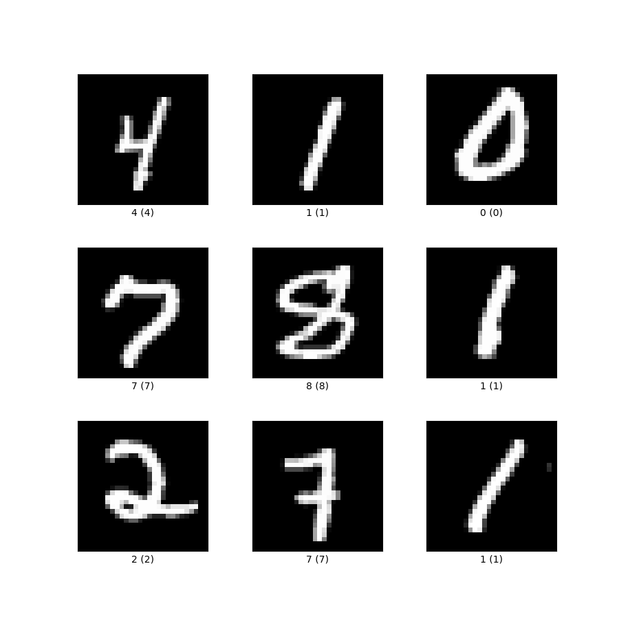source: https://storage.googleapis.com/tfds-data/visualization/fig/mnist-3.0.1.png

Each data point in the dataset is a 28 × 28 image, which is equivalent to 784 features that form the input dimension. These high dimensional representations are then compressed, as in many machine learning algorithms, and the compressed representations are used as input to a softmax layer for classification. Consider the following architecture for a linear classifier,

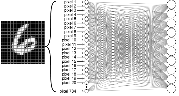source: https://ml4a.github.io/images/figures/mnist_1layer.png

Architecture

Layer 1

The input layer has 784 input nodes, where each node represents a single pixel value in the range of (0, 255) indicating the intensity or activation level of that pixel. We normalize the input by dividing by 255, reducing each node to the range (0, 1) before training, as this stabilizes the training process.

Hidden Layers

These layers compress the input information into condensed image representations, which are then used to predict the correct label of the given grayscale image. The hidden layer dimensions depend on your neural network design, but for a simple application like MNIST, we typically use the configuration with 2 hidden layers : 784 → 256 → 128 → 10 for deeper networks.

Note: The hidden layer dimensions are typically powers of 2 for computational efficiency, and progressively decrease in size as you move toward the output layer

Output Layer

The output layer converts the hidden layer representations into a probability distribution of the following form, Here, each probability represents how likely the input image belongs to that specific class. We then use cross-entropy loss to train our network.

Code

Now, we will explore how we can implement a network in PyTorch, first we need to import the dataset (lucky for us this dataset is available in torch and can be easily downloaded) and necessary libraries,

Part 1 - Import data and libraries

import torch
import torchvision
import torch.nn as nn
import torch.optim as optim
from torch.utils.data import DataLoader
import torchvision.transforms as transforms

import numpy as np
import matplotlib.pyplot as plt

device = torch.device('cuda' if torch.cuda.is_available() else 'cpu')

transform = transforms.Compose([
    transforms.ToTensor(),
])

train_dataset = torchvision.datasets.MNIST(
    root='./data',
    train=True,
    transform=transform,
    download=True
)

test_dataset = torchvision.datasets.MNIST(
    root='./data',
    train=False,
    transform=transform,
    download=True
)

The first few lines are used to import the necessary libraries.
device is used to determine if the training would be done on a CPU or a GPU, for something as simple as MNIST either is fine since its not too compute heavy.
transform is used to normalize the data
train_dataset, test_dataset are the datasets used to train the classifier, torchvision.datasets.MNIST is used to download the necessary data.
train = True / False decides if the data is for training or testing

batch_size = 64
train_loader = DataLoader(
    dataset=train_dataset,
    batch_size=batch_size,
    shuffle=True
)

test_loader = DataLoader(
    dataset=test_dataset,
    batch_size=batch_size,
    shuffle=True
)

print(f'Training samples: {len(train_dataset)}')
print(f'Test samples: {len(test_dataset)}')
print(f'Device: {device}')

batch_size is used to decide how many iterations 1 epoch will run for, to calculate how many iterations per epoch will run,
Consider the following example, num_train_samples = 60,000 (which is the actual number of training examples) and batch_size = 64
So each epoch runs for 938 iterations and if we have 10 epochs we would have a total 9380 iterations.
What is DataLoader? It is a utility class in the torch.utils.data module that loads and feeds data to the model during training or testing. It wraps the dataset into a iterable python object. We create two DataLoaders, one for training and one for testing.

Part 2 - Defining the linear model architecture

class LinearNN(nn.Module):
    def __init__(self, input_dim=784, hidden_dims=[256, 128], num_classes=10):
        super(LinearNN, self).__init__()
        
        # Input layer to first hidden layer
        self.fc1 = nn.Linear(input_dim, hidden_dims[0])
        self.relu1 = nn.ReLU()
        
        # First hidden layer to second hidden layer
        self.fc2 = nn.Linear(hidden_dims[0], hidden_dims[1])
        self.relu2 = nn.ReLU()
        
        # Second hidden layer to output layer
        self.fc3 = nn.Linear(hidden_dims[1], num_classes)
    
    def forward(self, x):
        x = x.view(x.size(0), -1)
        
        x = self.fc1(x)
        x = self.relu1(x)
        
        x = self.fc2(x)
        x = self.relu2(x)
        
        x = self.fc3(x)
        return x

model = LinearNN(input_dim=784, hidden_dims=[256, 128], num_classes=10).to(device)

print(model)
print(f'Total parameters: {sum(p.numel() for p in model.parameters())}')

Each model in PyTorch is defined as a Python class that inherits from nn.Module.
super() calls the parent class (nn.Module) constructor to properly initialize the module.
Each layer has (input, output) dimensions which help PyTorch maintain matrix consistency.
fc denotes a fully connected linear layer, created using nn.Linear(), which applies a linear transformation to the input which converts input dimension → output dimension using weight matrices.
ReLU is the activation function applied to intermediate output matrices, introducing non-linearity before passing to the next layer. It uses nn.ReLU().
forward() defines how forward propagation proceeds through the model:
x.view() flattens the image from (batch_size, 1, 28, 28) → (batch_size, 784)
x is then passed through the layers defined in init(), returning a vector of logits with shape (batch_size, 10) that can be converted into a probability distribution for training
We instantiate the model and send it to the device (CPU or GPU) for training using .to(device).

Part 3 - Training and testing

loss_fn = nn.CrossEntropyLoss()
optimizer = optim.Adam(model.parameters(), lr=0.001)

def train(model, train_loader, loss_fn, optimizer, device):
    model.train()
    running_loss = 0.0
    correct = 0
    total = 0
    
    for batch_idx, (images, labels) in enumerate(train_loader):
        images, labels = images.to(device), labels.to(device)
        
        optimizer.zero_grad()
        
        outputs = model(images)
        loss = loss_fn(outputs, labels)
        
        loss.backward()
        optimizer.step()
        
        running_loss += loss.item()
        _, predicted = torch.max(outputs.data, 1)
        total += labels.size(0)
        correct += (predicted == labels).sum().item()
    
    epoch_loss = running_loss / len(train_loader)
    epoch_acc = 100 * correct / total
    return epoch_loss, epoch_acc

nn.CrossEntropyLoss() defines the loss function used for training our model.
optim.Adam() is the optimizer used to minimize the cross-entropy loss by updating model parameters.
train() is a function defined to train the model given the (model, train_loader, loss_fn, optimizer, device).
First, we move the data and labels to the device (CPU or GPU).
Second, we clear the optimizer gradients from the previous iteration using optimizer.zero_grad().
Next, we run the forward pass to compute predictions, calculate the loss, then run the backward pass using loss.backward() to compute gradients for the current batch.
Next, We track the running loss and accuracy throughout the epoch to monitor that the model is learning and loss is decreasing.
Finally, we return the average epoch loss and epoch accuracy.

def test(model, test_loader, loss_fn, device):
    model.eval()
    running_loss = 0.0
    correct = 0
    total = 0
    
    with torch.no_grad():
        for images, labels in test_loader:
            images, labels = images.to(device), labels.to(device)
            
            outputs = model(images)
            loss = loss_fn(outputs, labels)
            
            running_loss += loss.item()
            _, predicted = torch.max(outputs.data, 1)
            total += labels.size(0)
            correct += (predicted == labels).sum().item()
    
    epoch_loss = running_loss / len(test_loader)
    epoch_acc = 100 * correct / total
    return epoch_loss, epoch_acc

Testing block is similar to the training block, the only difference is that it uses the test_loader instead of the train_loader

num_epochs = 10

for epoch in range(num_epochs):
    train_loss, train_acc = train(model, train_loader, loss_fn, optimizer, device)
    test_loss, test_acc = test(model, test_loader, loss_fn, device)
    
    print(f'Epoch [{epoch+1}/{num_epochs}]')
    print(f'Train Loss: {train_loss:.4f}, Train Acc: {train_acc:.2f}%')
    print(f'Test Loss: {test_loss:.4f}, Test Acc: {test_acc:.2f}%')
    print('-' * 50)

This is a simple loop that trains and tests the model and prints the loss and accuracy statistics.

Part 4 - Visualization

def visualize_predictions(model, test_loader, device, num_images=10):
    model.eval()
    images, labels = next(iter(test_loader))
    images, labels = images.to(device), labels.to(device)
    
    with torch.no_grad():
        outputs = model(images)
        _, predicted = torch.max(outputs, 1)
    
    fig, axes = plt.subplots(2, 5, figsize=(12, 5))
    for idx, ax in enumerate(axes.flat):
        img = images[idx].cpu().squeeze()
        ax.imshow(img, cmap='gray')
        ax.set_title(f'Pred: {predicted[idx].item()}, True: {labels[idx].item()}')
        ax.axis('off')
    plt.tight_layout()
    plt.show()

visualize_predictions(model, test_loader, device)

We get 10 random images from the test dataset and check if the trained models predictions are correct by displaying the images with their predictions

train_losses, train_accs = [], []
test_losses, test_accs = [], []

for epoch in range(num_epochs):
    train_loss, train_acc = train(model, train_loader, loss_fn, optimizer, device)
    test_loss, test_acc = test(model, test_loader, loss_fn, device)
    
    train_losses.append(train_loss)
    train_accs.append(train_acc)
    test_losses.append(test_loss)
    test_accs.append(test_acc)

fig, (ax1, ax2) = plt.subplots(1, 2, figsize=(12, 4))
ax1.plot(train_losses, label='Train Loss')
ax1.plot(test_losses, label='Test Loss')
ax1.set_xlabel('Epoch')
ax1.set_ylabel('Loss')
ax1.legend()
ax1.set_title('Loss Curves')

ax2.plot(train_accs, label='Train Accuracy')
ax2.plot(test_accs, label='Test Accuracy')
ax2.set_xlabel('Epoch')
ax2.set_ylabel('Accuracy (%)')
ax2.legend()
ax2.set_title('Accuracy Curves')
plt.tight_layout()
plt.show()

In this code block we are tracking loss and accuracy values so we can plot loss and accuracy curves and see how our model is learning by reducing loss through the epochs.

Why linear networks are not enough for visual machine learning?

There are a few reasons why linear networks fail to capture complex unstructured data like images with higher dimensions and even channels.

Flattening an image from 2D matrix to a 1D vector leads to a loss of spatial relationships (corners and centers have the same importance) which includes complex patterns, structures and textures.
The number of parameters explode in a linear architecture, consider the following example: A 224 x 224 RGB image and a single hidden layer with 512 neurons would require 224 × 224 × 3 × 512 = 77,070,336 parameters which makes it compute heavy and prone to overfitting.

What’s next?

Next we learn what a convolutional neural network is and how it works to combat information loss and parameter explosion.