From Recurrent Networks to Transformers, How Attention Changed Everything

This is part 2 of 2

But if we already have so many model architectures, why do we need Transformers?

The only reason why AI or machine learning in general has rattled so many heads can be attributed to the advent of GPUs. Older models like RNNs and LSTMs are inherently sequential, which makes them harder to train efficiently on parallel hardware. This is where the Transformer shines, it processes entire sequences in parallel, unlocking massive gains in speed and scalability. The transformer architecture was introduced in the 2017 paper - “Attention Is All You Need” (Vaswani et al., 2017) which introduced the attention mechanism which changed how we process natural language.

The Core Idea: Attention

So what is attention? It computes how much focus should one token give to another token, for that we calculate the scaled dot product between tokens and is given by,

$$\text{Attention}(Q, K, V) = \text{softmax}\left(\frac{QK^\top}{\sqrt{d_k}}\right)V$$

The softmax function takes a vector of real numbers and converts it into a probability distribution and is given by,

$$\text{softmax}(z_i) = \frac{e^{z_i}}{\sum_{j=1}^{n} e^{z_j}}$$

What are the variables Q, K, V

• Q (Query) : representation of the current token asking “what do I need?”
• K (Key) : representation of other tokens answering “what do I have?”
• V (Value) : actual information carried by the tokens.

The dot product and scaling factor given by,

$$\text{dot product = }{Q \cdot K^T}, \quad \text{scaling factor = }\sqrt d_k$$

Think of the dot product as a way for tokens to “measure how much they have in common each other.” The higher the similarity, the stronger the connection. But these raw scores can essentially “explode” so we scale them down.

In essence, attention determines how much of each value to use, effectively giving us a weighted percentage of the value to carry forward. Don’t worry we’ll go into a greater detail when we look at the actual architecture.

Tokens and Embeddings

Tokens: are IDs (indices) of words, subwords, or characters in the model’s vocabulary dictionary (dictionary refers to all the possible tokens the model can predict). Tokens don’t carry semantic meaning or context they’re in essence just numerical representations of words, subwords, or characters.

Example: Consider the following dictionary,

$vocab = \{the: 0, cat: 1, sat: 2, on: 3, tv: 4\}$

then the sentence “the cat” → tokens = [0, 1].

Token Embeddings: When we give semantic meanings to our token we get the token embeddings. This can be done in several ways, like using pre-trained embeddings using algorithms like word2vec or Glove.

In this paper they used learnt token embeddings which uses a randomized matrix initialized at the start of training and are learnt through training the model, take the token “the” for example and consider the following embedding matrix,

$$E = \begin{bmatrix} 0.2 & 0.1 & 0.4 & 0.7 \\ 0.9 & 0.3 & 0.5 & 0.8 \\ \ 0.1 & 0.6 & 0.2 & 0.4 \\ \ 0.5 & 0.7 & 0.1 & 0.3 \\ \ 0.8 & 0.2 & 0.9 & 0.6 \\ \end{bmatrix}_{5 \times 5}$$

the token “the” would be represented by the first row.

The Architecture - The Transformer Model

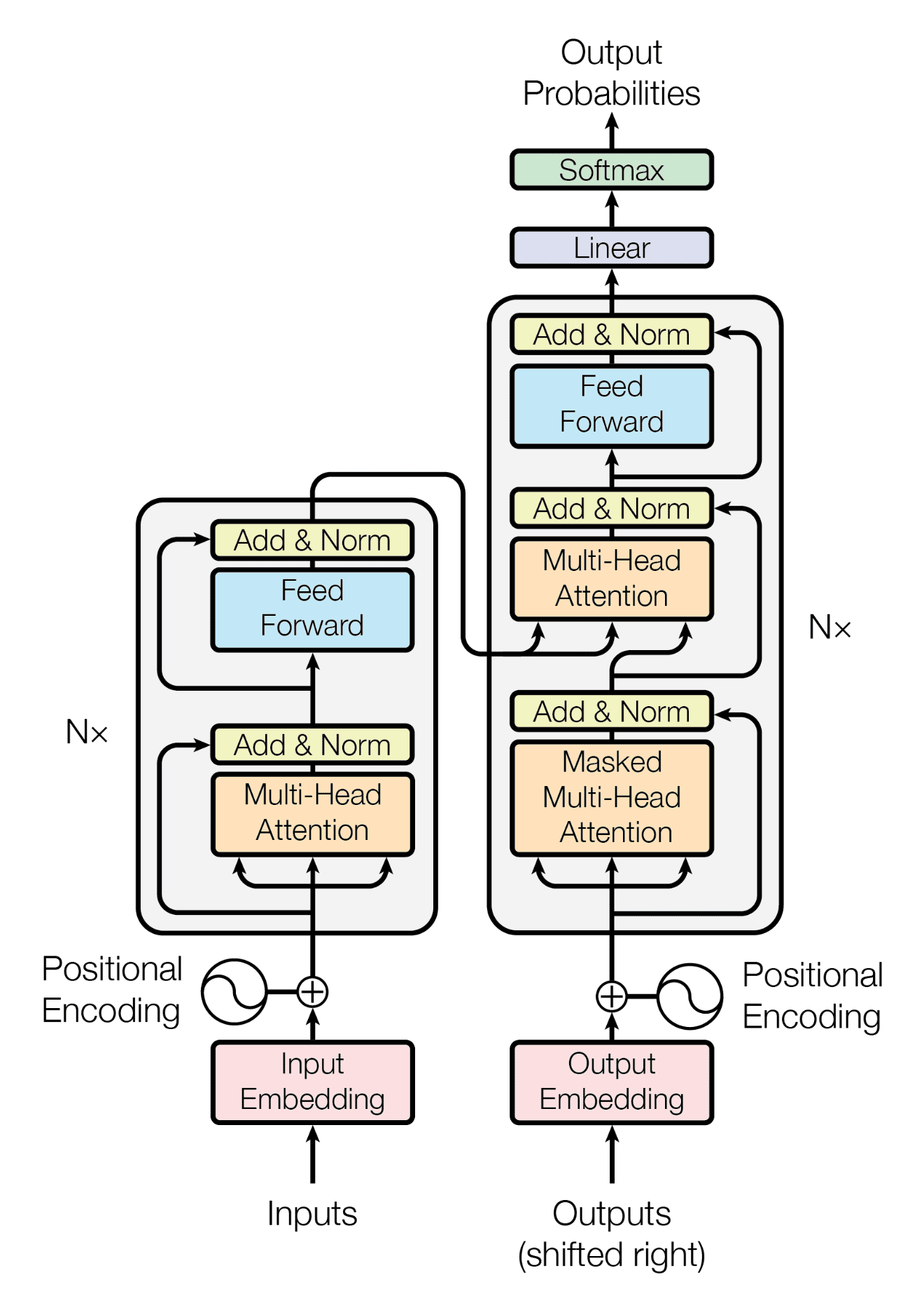
source: https://machinelearningmastery.com/wp-content/uploads/2021/08/attention%5Fresearch%5F1.png

Let’s breakdown each element of the architecture one-by-one

Left side or Encoder part of the transformer

Inputs and Input Embeddings

Input is the “sentence” passed through a tokenizer, which converts it into a string of tokens, these tokens are mapped to integer ID’s which correspond to their location in the models vocabulary, each token is then passed through the embedding layer which converts it into an embedding vector of size given by the following,

$$\text{Embedding Vector} = (1 \times d_{model}), \quad d_{model} = 512$$

In the original transformer architecture, each token is embedded into a 512-dimensional vector (d_model = 512), though this dimension varies across different implementations and models, for example DeepSeek R1 uses d_model = 7168, reason being that modern implementations of transformers aim to be more generalized so each embedding carries more information than the former implementation.

Positional Encoding

This is one of the reasons why the transformer shines, we add positional awareness to the token embedding we received in the previous step and the reason we can train a transformer faster is because we can use this positional information and context to parallelize using GPUs. This paper uses sinusoidal positional encodings which is given by,

$$\begin{matrix} PE_{even}{(pos, 2i)} = \sin\left(\frac{pos}{10000^{2i/d_{model}}}\right) \\ PE_{odd}{(pos, 2i+1)} = \cos\left(\frac{pos}{10000^{2i/d_{model}}}\right) \end{matrix}$$ $$\begin{matrix} i \in \text{dimension index} \\ pos \in \text{(0, 1, 2, ...) position of token} \\ \text{even indices use sine, odd indices use cosine} \\ n=10000 \text{ is a fixed scalar chosen by the authors} \end{matrix}$$

Consider the following sentence for example “I ate an apple”, for the token “ate” we would use the following hyper-parameters to produce a (1 x 512) positional vector that we can later use to add positional information,

$$\begin{matrix} d_{model} = 512 \\ i \in [0, 512), \ where \ i \in N\\ \text{even indices (2i) use sine} \\ \text{odd indices (2i+1) use cosine} \\ pos = 1 \ since, 2^{nd} \ token \ in \ sentence \end{matrix}$$

After computing for all the tokens we get a positional encoding matrix which is

(n x 512), where n defines the number of tokens in the sentence, in the example above our matrix would be of the form (4 x 512).

Note: These positional encodings are fixed in the original paper

Consider the following dimensions,

$$\begin{matrix} input = sentence \\ tokenizer \in (1 \times n) \\ token\_encodings \in (n \times d_{model}) \\ positional\_encodings \in (n \times d_{model}) \\ output \in (n \times d_{model}) \end{matrix}$$ $$\begin{matrix} n = \text{number of tokens} \\ d_{model} = \text{size of token embedding} \end{matrix}$$

Single Head Attention

As we discussed earlier, attention is when we compute how much focus should one token give to another token. Single head attention tries to compute how much each token focusses on every other token, lets take the following example : “I ate apple“ tokenized = [<sos>, I, ate, apple, <eos>], the single head attention output would look something like this,

$$A \approx \begin{bmatrix} 0.55, 0.10, 0.05, 0.20, 0.10 \\ 0.05, 0.60, 0.10, 0.15, 0.10 \\ 0.10, 0.05, 0.70, 0.10, 0.05 \\ 0.15, 0.10, 0.05, 0.60, 0.10 \\ 0.08, 0.12, 0.05, 0.10, 0.65 \end{bmatrix}_{5 \times 5}$$

Note: This is a random sample output and values may vary

1. The sum of rows = 1, since its a softmax operation.
2. It’s a (5 x 5) matrix since we’re processing a sentence with 5 tokens and each position in the matrix determine how token 1 “attends“ or “relate“ to token 2.
3. The values that are maximum in the row show how the 2 tokens “attend“ to each other and maximum implies that token 1 and token 2 in this specific head (more on that later) have the “best head specific relationship“

How to Calculate Attention

As we discussed earlier, attention is what drives this architecture home, we have already discussed the intuition behind Q, K, V matrices. Now let’s define dimensions and equations for the following: X, W (has been divided into 3 subsets) which is then used to calculate Q, K and V.

$$\begin{matrix} X \in (n \times d_{model}) \\ W_q \in (d_{model} \times d_q) \\ W_k \in (d_{model} \times d_k) \\ W_v \in (d_{model} \times d_v) \\ \end{matrix}$$ $$\text{for single head attention, }d_q = d_k = d_v = d_{model}$$ $$\begin{matrix} Q = X \times W_q \in (n \times d_q)\\ K = X \times W_k \in (n \times d_k) \\ V = X \times W_v \in (n \times d_v) \\ \end{matrix}$$

For single head attention we use following set of equations to calculate attention or “direction“ in which the token embedding should be shifted so its closer to other similar tokens which have some sort of relationship, be it meaning, semantic relationship, etc. Consider the following formula to calculate attention scores (A) and single head output (Z),

$$\begin{matrix} A = softmax\left(\frac{QK^T}{ \sqrt d_k}\right) \in (n \times n) \\ Z = A \cdot V \in (n \times d_v)\end{matrix}$$

where A and V were calculated earlier. We’ll next talk about about Multi Head Attention.

Multi Head Self Attention

In theory, multi head is the same as single head attention, the only difference is that we divide the single head to multiple heads, what does that mean and why do we need it? The model defined in the paper had $n = 8$, that means if $d_{model} = 512$, $d_k = 512 / 8 = 64$ or $d_k = d_{model} / n$, lets look at the dimensions in this specific case,

$$\begin{matrix} d_k = d_{model} / n, \quad n = \text{number of heads} \\ \\ X \in (n \times d_{model}) \\ W_q \in (d_{model} \times d_q) \\ W_k \in (d_{model} \times d_k) \\ W_v \in (d_{model} \times d_v) \\ \end{matrix}$$ $$\begin{matrix} Q_n = X \times W_q \in (n \times d_q)\\ K_n = X \times W_k \in (n \times d_k) \\ V_n = X \times W_v \in (n \times d_v) \\ \end{matrix}$$

Now we can calculate attention scores for all the different heads separately and stack them horizontally to produce the final output,

$$\begin{matrix} A_n = softmax\left(\frac{Q_nK^T_n}{ \sqrt d_k}\right) \in (n \times n) \\ Z_n = A_n \cdot V_n \in (n \times d_v) \\ \\ Z^o = [Z_1, Z_2, Z_3, \cdots, Z_8] \\ \text{MHA} = Z^o \cdot W^o \in (n \times d_{model})\end{matrix}$$

Note: The final weight matrix is used to compress all different head representations into a single matrix.

Why do we need multiple heads?

The reason why we would need more than 1 head is because multiple heads can capture better semantic representations of the tokens, think of it this way, why do we need more layers in a neural network or why do we need more nodes in a layer of a neural network, similarly we need multiple heads to capture different representations of the tokens.

Add and Normalize

The next step is to add the residual signal (the signal or data that was not passed through the multi head computation) and then layer-normalizing it,

$$out = LayerNorm(x + multi\_head\_attention(x)), \quad x = \text{original signal}$$

What is LayerNorm? Normalizes across features (columns) of each sample (not across the batch, unlike BatchNorm). It is given by the following,

$$\begin{matrix} y = γ \odot \frac{x − \mu}{\sqrt{\sigma^2 + ε}} + β \\ \mu = \frac{1}{d_{model}} \sum_{j=1}^{d_{model}} x_j\\ \sigma^2 = \frac{1}{d_{model}} ∑_{j=1}^{d_{model}} (x_j − \mu)^2 \end{matrix}$$

1. ε is a small constant for numerical stability (fixed hyper-parameter).
2. γ (gamma), β (beta) are learnt with training and are not fixed.

Feed Forward Neural Network

Why do we need a neural network and what does it do? We use it to add non linearity to the model which helps it learn complex objective functions and it is point-wise meaning it changes the hidden state for each token independently which means that it respects the positional information of each token even when it is passed as a matrix to parallelize the process. Usually the hidden layer of the FFNN is 4 times the d_model, now lets look at the dimensions and equations for this process,

$$\begin{matrix} input = x \\ z_1 = \phi(xW_1 + b_1) \\ \hat y = z_1W_2 + b_2 \\ \text{Note: } \phi \text{ is an activation function} \end{matrix}$$ $$\begin{matrix} x \in (n \times d_{model}) \\ W_1 \in (d_{model} \times d_{ff}) \\ b_1 \in (1 \times d_{ff}) \\ \\ z_1 \in (n \times d_{ff}) \\ W_2 \in (d_{ff} \times d_{model}) \\ b_2 \in (1 \times d_{model}) \\ \\ \hat y \in (n \times d_{model}) \\ \end{matrix}$$

1. Common activation functions used are ReLU, GELU, SwiGLU
2. After transforming the signal using the neural network we follow the same add and normalize step to produce the outputs.
3. We use the *FINAL* output from the *last encoder block* to calculate cross attention, more on that later.

Right side or Decoder part of the transformer

Outputs (Shifted right)

Outputs are the tokens we pass to the decoder and they are shifted by one token. Why do we do that? Well we need to start from something and during training we have the whole sentence we want to generate, and we don’t wanna cheat with generation so we shift the outputs by one token. Take the sentence “I ate an apple“ for instance, after tokenizing and shifting it becomes [“<sos>”, “I”, “ate”, “an”, “apple”]. This means that we use “<sos>” to predict “I”, “<sos> I” to predict “ate“, and so on. The property of LLMs to produce a single token at a time is called auto-regressive.

We pass the whole sentence which is right shifted to the decoder block, we do this for efficient training and we add a mask on the future tokens so the model doesn’t cheat during the training process, more on that later.

Embedding and Positional Encoding

The sentence is tokenized, converted into token embeddings and positional encodings are added to the vector just like the encoder block, consider the following dimensions,

$$\begin{matrix} input = \text{sentence right shifted} \\ tokenizer \in (1 \times n) \\ token\_encodings \in (n \times d_{model}) \\ positional\_encodings \in (n \times d_{model}) \\ output \in (n \times d_{model}) \end{matrix}$$

Note: Encoder and Decoder can have the same value of n even after shifting, because in practice we pad the sequences to a maximum length so we can consider the sizes to be n instead of n+1 for simplicity.

Multi Head Masked Attention

This is similar to “self attention“ where each token is exposed to every other token in the sequence, the major difference is we mask the output of the future token so the model cannot cheat its way to a good prediction.

How do we do it? We simply add -∞ to the future tokens while calculating the attention scores for the sequence.

Consider the following dimensions for masked attention,

$$\begin{matrix} X \in (n \times d_{model}) \\ W_q \in (d_{model} \times d_q) \\ W_k \in (d_{model} \times d_k) \\ W_v \in (d_{model} \times d_v) \\ \end{matrix}$$ $$\begin{matrix} Q = X \times W_q \in (n \times d_q)\\ K = X \times W_k \in (n \times d_k) \\ V = X \times W_v \in (n \times d_v) \\ \end{matrix}$$

Now consider the following equations,

$$\begin{matrix} A_n = softmax\left(\frac{Q_nK^T_n + M}{ \sqrt d_k}\right) \in (n \times n) \\ M_{i,j} \in \begin{cases} 0 & \text{if } j \le i \\ -\infty & \text{if } j \gt i \end{cases} \\ \\ Z_n = A_n \cdot V_n \in (n \times d_v) \\ Z^o = [Z_1, Z_2, Z_3, \cdots, Z_8] \in (n \times d_{model}) \\ \\ \text{MHMA} = Z^o \times W^o \in (n \times d_{model}) \end{matrix}$$

1. Similar to multi head self attention the final weight matrix is used to compress all different head representations into a single matrix.
2. After transforming the signal using the multi head masked attention step we follow the same add and normalize step to produce the outputs.

Consider the following transformation of attention scores for following example : “I ate apple“, tokenized = [, I, ate, apple, ], the attention output would look something like this

$$A \approx \begin{bmatrix} 0.55, 0.10, 0.05, 0.20, 0.10 \\ 0.05, 0.60, 0.10, 0.15, 0.10 \\ 0.10, 0.05, 0.70, 0.10, 0.05 \\ 0.15, 0.10, 0.05, 0.60, 0.10 \\ 0.08, 0.12, 0.05, 0.10, 0.65 \end{bmatrix}_{5 \times 5}$$

after adding a mask and softmax is applied,

$$A_{masked} \approx \begin{bmatrix} 1.00 & 0 & 0 & 0 & 0 \\ 0.40 & 0.60 & 0 & 0 & 0 \\ 0.32 & 0.33 & 0.35 & 0 & 0 \\ 0.25 & 0.20 & 0.25 & 0.30 & 0 \\ 0.20 & 0.10 & 0.10 & 0.20 & 0.40 \\ \end{bmatrix}_{5 \times 5}$$

Note: This is a random sample output and values may vary

Multi Head Cross Attention

what is cross attention and why do we need it? Cross attention is when we use information, i.e K, V matrices from the encoder and Q matrix from the decoder to produce the attention matrix. To truly understand why we need it, we need to understand what each part of the architecture does, the encoder or the left part creates semantically aware and dense token representations to capture the meaning and / or context of the input sequence and these representations are used by the decoder or the right part to generate better token outputs.

In essence, cross-attention is how the decoder “looks at” the entire source sentence to inform each prediction, rather than generating based solely on previous outputs.

Consider the following dimensions for multi head cross attention,

$$\begin{matrix} X \in (n \times d_{model}) \\ W_q \in (d_{model} \times d_q) \\ W_k \in (d_{model} \times d_k) \\ W_v \in (d_{model} \times d_v) \\ \end{matrix}$$

Now consider the following equations,

$$\begin{matrix} Q_{dec} = X_{dec} \times W_q \in (n \times d_q)\\ K_{enc} = X_{enc} \times W_k \in (n \times d_k) \\ V_{enc} = X_{enc} \times W_v \in (n \times d_v) \\ X_{dec} = \text{output from decoder or decoder context} \\ X_{enc} = \text{output from encoder or encoder context} \end{matrix}$$ $$\begin{matrix} A_n = softmax\left(\frac{Q_{dec}K^T_{enc}}{ \sqrt d_k}\right) \in (n \times n) \\ Z_n = A_n \cdot V_n \in (n \times d_v) \\ Z^o = [Z_1, Z_2, Z_3, \cdots, Z_8] \in (n \times d_{model}) \\ \\ \text{MHCA} = Z^o \times W^o \in (n \times d_{model}) \end{matrix}$$

1. Similar to multi head self attention the final weight matrix is used to compress all different head representations into a single matrix.
2. After transforming the signal using the multi head cross attention step we follow the same add and normalize step to produce the outputs.

Feed Forward Neural Network

Similar to the encoder, each decoder block also has a FFNN, it is used to add non-linearity and it is first expanded and then compressed, which allows for a richer, more expressive transformations.

$$\begin{matrix} input = x \\ z_1 = \phi(xW_1 + b_1) \\ \hat y = z_1W_2 + b_2 \\ \text{Note: } \phi \text{ is an activation function} \end{matrix}$$ $$\begin{matrix} x \in (n \times d_{model}) \\ W_1 \in (d_{model} \times d_{ff}) \\ b_1 \in (1 \times d_{ff}) \\ \\ z_1 \in (n \times d_{ff}) \\ W_2 \in (d_{ff} \times d_{model}) \\ b_2 \in (1 \times d_{model}) \\ \\ \hat y \in (n \times d_{model}) \\ \end{matrix}$$

Note: After transforming the signal using the neural network we follow the same add and normalize step to produce the outputs.

Final Step : Prediction

This is one of the easier parts of the architecture, the output matrix of the final decoder block is flattened out to an output layer vector of size $(1, vocabulary\_size)$ and each node in the final layer represent the $token\_ids$. The final layers output is passed through a softmax function to produce probabilities and the one with the highest probability is chosen to be the output token.

During training cross-entropy loss is calculated between the predicted token and the ground truth token.

During inference, the model generates the token with the highest probability and feeds the previous sequence + predicted token back to the decoder to generate more tokens (auto-regressive).

Consider the following dimensions and equations for the prediction step,

$$\begin{matrix} input = X^{out}_{dec} \in (n \times d_{model}) \\ W_L \in (d_{model} \times |V|) \\ \\ linear = X^{out}_{dec} \times W_L \in (n \times |V|) \\ output = softmax(linear) \in (n \times |V|) \end{matrix}$$

Consider the following example for vocab_size = 4 and 2nd prediction,

$$\begin{matrix} actual = \begin{bmatrix} 1 & 0 & 0 & 0 \\ 0 & 0 & 1 & 0 \end{bmatrix}_{2 \times |V|} \\ \\ predicted = \begin{bmatrix} 0.6 & 0.1 & 0.1 & 0.2 \\ 0.1 & 0.1 & 0.7 & 0.1 \end{bmatrix}_{2 \times |V|} \end{matrix}$$

Now we can use these to train our network, and as we produce more tokens we add more rows to the matrices.

Encoder: Used to build rich, context-aware representations from an input sequence, enabling downstream understanding or prediction tasks (e.g., BERT for classification and embedding).

Decoder: Used to generate (predict) output tokens in an autoregressive fashion, conditioned on previous tokens and (optionally) additional context, such as encoder-decoder transformers (e.g., GPT for generation, T5 for seq2seq tasks).